School Finance 101: Toward a Consensus Approach to Evaluating State School Finance Systems! (and Dumping the Others!)
")
Over the past decade, there has been an emerging consensus regarding state school finance systems, money and schools. That consensus is supported by a growing body of high-quality empirical research regarding the importance of equitable and adequate financing for providing quality schooling to all children. As guideposts for this new and improved annual report on state school finance systems, we offer the following five core principles:
- The level and distribution of school funding matters;
- Achieve higher outcomes and a broader array of outcomes often requires additional resources and may require substantial additional resources;
- Achieving competitive student outcomes depends on adequate school resources, including a competitively compensated teacher workforce;
- Closing achievement gaps between children from rich and poor neighborhoods requires progressive distribution of resources targeted toward children with greater educational needs;
- Both the adequacy of students’ outcomes and improving the equity of those outcomes are in our national interest.
But US public schooling remains primarily in the hands of states. On average, about 90 percent of funding for local public school systems and charter schools comes from state and local tax sources. How state and local revenue is raised and distributed is a function of seemingly complicated calculations usually adopted as legislation and often with the goal of achieving more equitable and adequate public schooling for the state’s children.
Core Principles of Funding Fairness
Beginning in 2010, in collaboration with the Education Law Center of New Jersey, we laid out a methodology and series of indicators for comparing state school finance systems using available national data sets. With support from the William T. Grant Foundation, we dramatically expanded our analyses and developed publicly accessible district and state level databases – The School Funding Fairness Data System. More recently, we have combined our data with those of the Stanford Education Data Archive to estimate a National Education Cost Model. Concurrently, we have begun to expand our state funding equity analyses to include public two-year colleges, applying similar methods of analysis.
We based the original method on the relatively straightforward premise that:
…all else equal, local public school districts serving higher concentrations of children from low income backgrounds should have access to higher state and local revenue per pupil than districts serving lower concentrations of children in poverty.
By “all else equal” we mean that comparisons of resources between lower- and higher-poverty school districts are contingent on differences in labor costs and other factors, such as economies of scale and population density. State school finance systems should yield progressive distributions of state and local revenue, which should translate to progressive distributions of current spending per pupil, progressive distributions of staffing ratios, and competitive teacher wages. Other organizations, including the Urban Institute, have adopted similar approaches, acknowledging the basic need for funding distributions that are progressive with respect to child poverty.[1] Of course, progressiveness alone may not be sufficient. Progressive distributions of funding must be coupled with sufficient overall levels of funding to achieve the desired outcomes. No state has a perfect school finance system, but a few states stand out as providing sufficient levels of funding and reasonable degrees of progressiveness. Massachusetts and New Jersey are among the best examples.
There is now broad agreement between scholars and organizations across the political and disciplinary spectra that school districts serving higher need student populations – those with higher poverty rates in particular – require not the same, but rather moreresources per pupil than districts serving lower need student populations. In other words: state school finance systems should channel more funds toward districts with higher levels of student poverty, because that’s where those funds are needed the most. The equity measures produced in our report, those produced by the Urban Institute, and those produced by the Education Trust all acknowledge this basic goal of state school finance systems and framing of equal educational opportunity.
Consensus indicators
Drawing on our past reports and convenings with representatives of various interest groups and organizations involved in state school funding deliberations, we propose the following Consensus indicators for comparing and evaluating state school finance systems.
- Educational Effort: The share of a state’s economic capacity which is spent on elementary and secondary education (and/or postsecondary education) in combined state and local resources.
- State economic capacity can and should be measured by both a) gross domestic product, state and b) aggregate personal income.
This indicator provides a policy relevant representation of the effort a state is putting forth to fund its public education systems. It makes less sense, for example, to evaluate the share of state total revenue (state budget) allotted to schools, because some states simply choose not to levy sufficient taxes to support any quality public services. Effort is a policy choice, representing both the choice to levy sufficient taxes and the priority placed on public education. Combined with the adequacy of spending levels, the effort indicator allows us to determine which states lag behind in spending because they simply lack capacity, versus those that lag behind because they don’t put up the effort.
Adequacy (Spending Levels):
- Equated spending levels: Per pupil spending (or revenue) levels for districts a) of efficient scale (>2,000 pupils), comparable population density, national average competitive wages and at specific rates of student need (child poverty).
- Equated spending to common outcome goals (NECM): Per pupil spending levels adjusted fully for the costs of achieving common outcome goals, wherein cost adjustment involves consideration of a) regional variation of competitive wages, b) economies of scale and population density, c) student needs (child poverty, adjusted for regional income variation), and d) assuming districts produce outcomes at current national average efficiency.
The first of these indicators merely compares equated spending or revenue levels for otherwise similar school districts. That is, what does a school district of efficient scale and average density, national average wages, with 10% children in poverty spend in New Mexico versus New York? Such adjustment is more complete than merely dividing current spending by a regional wage adjustment factor, as it also accounts for the higher average spending in states with larger shares of children in small, sparsely populated districts. This approach also compares spending for districts at similar rates of child poverty.
The second of these indicators compares spending based on the costs of achieving existing (prior year) national average outcomes, given the same contextual cost factors, and modeling the relationship between spending and district level outcomes over several years. This approach allows us to more completely characterize the “relative” adequacy of existing spending toward achieving common outcome goals, from one state or district to another, across the nation.
- Progressiveness: The relationship between available resource quantities (per pupil spending, revenue, teachers per 100 pupils, etc.) and child poverty across schools or districts. A progressive system is one in which schools or districts serving higher shares of children from low income family backgrounds (all else equal) have greater quantities of resources available to them. Progressiveness should be both substantial and systematic:
- Substantial: That the ratio or slope of the relationship between resource quantities in high poverty to low poverty schools or districts is large (e.g. high poverty districts have 50% or more resources per pupil than low poverty districts). This can be measured by either the high/low poverty ratio or slope of the relationship between poverty and resources across schools or districts.
- Systematic: That the relationship between schools’ or districts’ student population needs is systematic across districts, falling in a predictable pattern whereby districts serving higher need student populations have more resources per pupil. This can be evaluated by the amount of variation in resources explained by variation in student needs (r-squared or partial correlation).
- Competitive teacher compensation: In order to recruit and retain a high-quality teacher workforce, the wages paid to teachers must be comparable to those of non-teachers holding similar levels of education, at similar ages (or experience levels) and for a certain amount of time worked.
It is not necessarily the case that teacher wages should be at 100% parity with those of non-teachers, or higher or lower than that. Rather, if we expect to maintain a teacher workforce of constant quality, the teacher to non-teacher wage should stay constant, not fall further behind. Similarly, the gap, if any, should be similar across settings to achieve comparable recruitment and retention. So, we compare teacher wage competitiveness in relative terms, across states and over time. We refer in our reports to a Salary Parity Ratio, which compares teacher to non-teacher wags, based on Census data, at constant degree level, age, hours per week and weeks per year. The Economic Policy Institute takes a similar approach with Bureau of Labor Statistics data to compare weekly wages of teachers and non-teachers at constant degree levels.
[1] Matthew M. Chingos and Kristin Blagg, Do Poor Kids Get Their Fair Share of School Funding? (Washington, DC: Urban Institute, 2017).
Comparison to Other Indicators
In this brief, we compare our indicators with those of other organizations which seek to characterize and evaluate state public school finance systems and teacher wages. It was our original intent in designing and producing our indicators that they would be more comprehensive, more precise and more meaningful than other measures of state school finance systems. At the time of our first report, two other reports dominated the public discourse on state school funding inequity – Education Week’s Quality Counts and the Education Trust Funding Gap report. Education Week has continued to rely on largely the same indicators we critiqued in our original technical report in 2010.[1] We revisit problems with those indicators here.
The Education Trust has sporadically revisited their funding gap report, measuring differences in per pupil revenue between higher and low poverty, higher and lower racial minority concentration districts. Their initial report prompted our efforts to pursue greater precision and accuracy in characterizing state school finance systems along similar conceptual lines. In the mid-2000s, Education Trust produced Funding Gap reports which seemed to suggest that Kansas was among those states where districts higher in child poverty spent, on average more than lower poverty districts. Two complicating factors led to this mischaracterization, both related to the fact that Kansas has large shares of children in very small, rural districts. First, poverty rates tend to be overstated in rural areas, compared to urban areas.[2] Second, Kansas’ state school finance formula provides substantially greater funding to very small districts to compensate for their lacking economies of scale. In fact, the state over-subsidizes (or did at the time) scale related costs.[3] So, in Kansas, very small rural districts with overstated poverty do spend more than lower poverty districts. But after accounting for differences in poverty measurement and in district size, this difference is muted or negated if not reversed (in most data years).
At issue in any evaluation of per pupil resource variation is the sorting out of resource variation that is intended and based on differences in costs and needs versus resource variation that is random, inequitable or otherwise purposefully inducing inequities. Major factors influencing the cost of providing equitable and adequate educational programs and services are well understood but overlooked in most existing reports on school funding equity.[4] Major factors include the following:
- Input prices:
- Competitive Wage Variation
- Geographic Factors:
- Economies of scale
- Population Sparsity
- Student Needs:
- Child Poverty
- Disability (by Severity)
- Language proficiency
Most recent reports on school funding do make use of Lori Taylor’s Education Comparable Wage Index as a basis for calculated regionally cost adjusted per pupil revenue or spending. But all others (other than ours) ignore entirely differences in economies of scale and population sparsity, and the intersection between the two. Some reports will also assign “pupil weights” as cost adjustments for student needs, such as assuming it costs an additional 50% for each low income child. However, where states allocate more than 50% additional funding for low income children, those variations are assumed to be inequitable variations even if they come closer to addressing the actual costs of achieving common outcomes for low income children. Unfortunately, no single common weighting scheme suffices for adjusting student need related costs.
Table 1 summarizes the measures, their intended purposes and cost factors which are accounted for in their estimation. Education Week’s Quality Counts (EWQC) report remains the lone holdout in applying especially dated methods and measures. First, the EWQC report relies on arbitrary pupil need weights to adjust for “costs” associated with specific student populations. EWQC also uses the Education Comparable Wage Index to adjust for regional variation in competitive wages for teachers. Then, EWQC estimates a series of measures of variation in per pupil spending after adjusting that spending for student needs and regional wage variation.
The first is the coefficient of variation, which is simply the standard deviation of per pupil spending expressed as a percent of the mean spending. Assuming a normal distribution, a CV of .10 would indicate that about 2/3 of children (assuming the analysis to be student weighted) attend districts within 10% of average per pupil spending. The “restricted range” is the difference in per pupil spending between the district attended by the 95%ile pupil and the district attended by the 5%ile pupil (ranked from highest to lowest per pupil spending). A significant shortcoming of both of these measures, when using arbitrary weights to adjust for student need costs, is that some variation in spending reflected in the CV might actually be a function of the state targeting resources according to need more aggressively than the weight chosen by Ed Week. Additional variation in spending might occur due to other legitimate cost factors like scale and sparsity which aren’t accounted for at all in the EWQC report.
The McLoone Index is a measure which relates the average spending on students in the lower half of the school spending distribution, as a percent of spending on the median pupil. That, it’s a measure of the extent to which the bottom half is leveled up toward the median. The meaningfulness of this measure is contingent on the adequacy of that median. In very low spending states, the median child may attend a woefully inadequately funded district. A state can achieve a relatively high McLoone Index, for example, if half or nearly half of the children in a state attend one or a few very large districts whose per pupil spending is near the median. And again, this measure like the others does not fully sort out “good (equitable) variation” from inequitable variation. The McLoone Index, while perhaps useful in its day, provides relatively limited information for understanding modern state school finance policies.
EWQC also includes two measures of spending levels intended to imply “adequacy” of funding. The first is a measure of the share of children in each state attending districts at or above the national average per pupil spending. The second is a “spending index” which is kind of like a national McLoone Index, but measured against the national mean rather than median. The spending index evaluates “the degree to which lower-spending districts fall short of that national benchmark. In states that scored 100 percent, all districts met or cleared that bar.”
Most recently the Urban Institute (UI) developed a school funding “progressiveness” index, which parallels the conceptual framing of our own index. The Urban Institute Index adjusts per pupil revenue for regional variation in competitive wages. Then, the Urban Institute calculates for each state, and average revenue per pupil figure for children in poverty (average weighted by U.S. Census poverty count) and an average revenue per pupil for children NOT in poverty. The gap between the two is the progressiveness measure (which could as easily be expressed as a ratio rather than dollar gap). States where the poverty weighted per pupil revenue figure is higher (gap>0) are progressive and vice versa. This approach has a few key differences from ours.
- First, Urban Institute simply divides per pupil revenues by the regional wage index, rather than regressing revenues against the index (reducing the influence of the regional cost adjustment).
- Second, Urban Institute does not adjust Census Poverty Rates for regional variation in income, as we do.[5]
- Third, Urban Institute makes no attempt to account for economies of scale, population sparsity or the interaction between the two.
But, the UI conceptual approach is consistent with ours and should reflect similar patterns across states, differing most among states with large shares of children attending, small, sparsely populated and remote rural districts.
Table 1
Comparison of Indicators
| Source | Measure | Intended | Accounting for Equitable Variation |
| Education Week/ Quality Counts | Coefficient of Variation | Equity | Arbitrary “weights” to adjust for student needs
ECWI to adjust for regional wage variation |
| Restricted Range | Equity | ||
| McLoone Index | Equity of lower half (“adequacy”) | ||
| % Students in Districts above National Average PPE | adequacy | ||
| Per-pupil spending levels weighted by the degree to which districts meet or approach the national average for expenditures (cost and student need adjusted) | adequacy | ||
| Urban Institute | Progressiveness | Equity | Child poverty
ECWI to adjust for regional wage variation ECWI adjusted mean for children in poverty (poverty weighted) vs. those not in poverty |
| Funding Fairness | Progressiveness | Equity | Modeled “predicted values” accounting for:
Child poverty (adjusted for regional wage variation) Wage variation (ECWI) Economies of scale Population density |
| Level | Adequacy | ||
| NECM | Level (by poverty quintile) | Adequacy (and equity) | Modeled “predicted values” accounting for:
Child poverty (adjusted for regional wage variation) Wage variation (ECWI) Economies of scale Population density Grades served Efficiency factors Constant outcomes |
Most recently, we have added to our catalog of indicators, measures of relative “adequacy” from our National Education Cost Model. These model-based estimates not only account for all of the “cost factors” included in our Funding Fairness Models, but also attempt to fully equate spending with respect to common outcome goals. That is, how much does it cost, from one location to another, one child to another, to achieve common outcome goals? And how far above or below those cost predictions are current spending levels? In the process, we assign common efficiency expectations for all districts. That is, costs of achieving the outcome goal in question are based on an assumption that each district achieves those outcomes at the efficiency level of the average district.
Table 2 compares our approach to constructing an index of the competitiveness of teacher wages to the approach used by Sylvia Allegretto with the Economic Policy Institute. Both indices compare the average wages of teachers, at constant degree levels, to wages of non-teachers. The EPI index compares weekly wages of teachers to non-teachers holding a bachelors or master’s degree using data from the Bureau of Labor Statistics, Current Population Survey.[6] Our approach uses data from the American Community Survey of the U.S. Census Bureau and estimates a model of wages for teachers and non-teachers, controlling for their age, degree level (including masters and bachelors recipients only), hours worked per week and weeks worked per year.
Table 2
Comparison of Wage Competitiveness Measures
| Source | Measure | Data Source | Controls |
| EPI (Allegretto) | Teaching Penalty = teacher weekly wage / non-teacher weekly wage (by degree level) | Bureau of Labor Statistics Current Population Survey | Time at work (unit=week)
Degree level |
| Funding Fairness | Wage Parity = teacher wage / comparable non-teacher wage | American Community Survey | Age
Degree level Hours per week Weeks per year |
Equity Measures
Here, we take a look at the relationships between our indicators and those of others, first focusing on indicators intended to represent equity. Figure 1 shows the relationship between the EWQC coefficient of variation an our measure of spending progressiveness – that is, to what extent is spending variation positively associated with child poverty? How much higher (or lower) is spending per pupil in higher poverty versus lower poverty districts.
EWQC finds similar degrees of variation (similar CV) for Pennsylvania, Illinois, New Jersey and Massachusetts. If anything, EWQC’s CV suggests that Massachusetts and New Jersey are slightly less equitable than Pennsylvania or Illinois (further to the right, higher CV, more variation). But, vertically, PA and IL sit nearer the bottom around or below 1.0, indicating that both of these states have regressive distributions of spending with respect to poverty whereas MA and NJ have progressive distributions of spending. In fact, it is the progessiveness itself that is handicapping MA and NJ on the EWQC measure, yielding the erroneous conclusion. In part, the “variation” reflected in the CV in an enrollment-weighted average is reduced in PA and IL by the presence of very large urban districts (Chicago and Philadelphia) because the calculation assumes all children within those districts receive precisely the same per pupil resources.
Figure 1

EWQC does separately relate property wealth to district spending to determine the “neutrality” of spending from wealth, wherein the preferred condition is one where there exists little or not relationship between district taxable property wealth and revenue or spending per pupil. But Figure 2 shows that even this measure has little or no relationship to our more meaningful, more accurate and precise progressiveness measure. The neutrality measure does pick up the inequities of the Illinois system, but continues to place Massachusetts between Illinois and Pennsylvania despite Massachusetts having a decisively more progressively funded system. Indeed, these measures are designed to show different things, and thus they do. But in an era of information overload, it would be wise for us to select and emphasize that subset of measures which most accurately convey what we really need to know about state school finance systems.
That is, is the overall level of funding sufficient to achieve desired outcomes? And do children and setting with greater needs and costs have sufficiently more resources to have equal opportunity to achieve those outcomes? (are the systems sufficiently progressive?) Whether there remains some relationship to taxable property may be unimportant, or a mere artifact of the distribution of taxable wealth (including high value undesirable properties like utilities, refineries or oil fields).
Figure 2

Figure 3 provides a clearer view of per pupil spending (centered around labor market means) and child poverty rates (centered around labor market means) for Massachusetts, New Jersey, Illinois and Pennsylvania. Figure 3 shows specifically that New Jersey per pupil spending tilts upward as poverty increases. That is, it’s progressive. Massachusetts is relatively flat, but Boston (the large circle) is higher in the distribution, creating an average upward tilt, but less systematic than New Jersey. Pennsylvania, by contrast is systematically regressive, with the largest district Philadelphia having very high poverty and low spending. In Illinois, Chicago sits marginally below the average for its labor market on spending, and also with high poverty. Among these states, New Jersey is clearly most equitable, with Massachusetts second, Illinois a distant third and Pennsylvania at rock bottom. But the EWQC equity indicators convey and entirely different – incorrect – conclusion.
Figure 3

Figure 4 displays the relationship between the Urban Institute progressiveness measure and our progressiveness measure for state and local revenue per pupil. The relationship is weaker than we might expect, but mainly because so many states are clustered together near the center of the distribution. Figure 4 shows that New Jersey is in fact progressive by both measures and Illinois is regressive by both measures, in contrast with the EWQC equity indicators which suggested little difference in equity between New Jersey and Illinois. Massachusetts is also identified as progressive by both indicators.
Figure 4

Adequacy Measures
Figure 5 compares the McLoone Index to our measure from our National Education Cost Model in which we compare current spending to the spending predicted to be needed to achieve national average outcomes in reading and math. There exists little relationship between the two, and the relationship that does exist tilts in the wrong direction. A higher McLoone index is intended to indicate more adequate funding. That is, that the bottom half is closer to the median. But, states with a higher McLoone index seem to have, on average, lower spending relative to spending needed for average outcomes. This finding might be intuitive if states with especially low spending effectively “bottom out” on spending. That is, the bottom half lies at a bare minimum threshold which is also very close to the median – which is very low. This is the case, for example in Arizona and Mississippi. Because this is the case, the McLoone Index is an especially poor indicator for evaluating adequacy (or equity) of spending. Notably, Vermont and New Hampshire, which have very low McLoone indices also have among the most adequate average spending, largely because they hare relatively low need student populations coupled with relatively high average per pupil spending.
Figure 5

Figure 6 relates the proportion of children attending districts with above national average spending to our measure of the relative adequacy of current per pupil spending (toward achieving national average outcomes). Here at least we see a modest positive relationship. States with more children attending districts with above average spending do, on average tend to have more adequate spending by our more precise and accurate measure. But if we choose to focus on adequacy for high poverty districts with our measure, as we have done here, we can see that children in high poverty districts in states like Pennsylvania actually only spend 60% of what they would need to spend to achieve average outcomes, even though the state share of children attending districts at or above national average spending is near 100%. By contrast, using our measure, spending in Kansas and Iowa is near the level needed for national average outcomes, even though only 20% of children attend districts at or above national average spending.
Figure 6
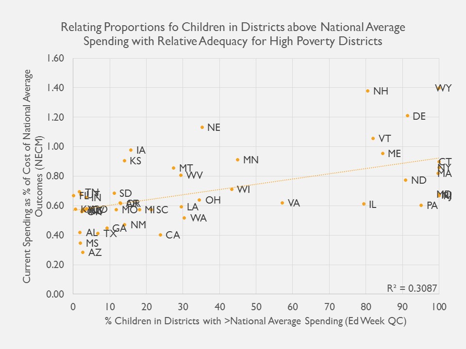
Figure 7

Figure 7 relates our measure of spending relative adequacy – spending relative to the cost of achieving national average outcomes in reading and math – to the EWQC spending index. There exists a modes relationship between the two, which makes sense in that weighted average spending relative to national averages should be at least somewhat associated with the relative adequacy of funding toward achieving national average outcomes. But even then there are some significant disconnects. The EWQC spending index rates Utah as similar to Arizona and Vermont as similar to Pennsylvania. But our measure of relative adequacy for high poverty schools differs significantly between these pairings, primarily because we account more fully for costs associated with the student populations served.
Figure 8 shows the position of Vermont and Pennsylvania school districts, by their poverty rate, on our measure of relative adequacy. The figure includes only unified K12 districts with greater than 500 enrolled students. All districts nationally are in the beige background. The horizontal red line indicates the “cost” of achieving national average outcomes (or $0 gap). In Pennsylvania, several districts, many of them very large districts including Allentown, Reading and Philadelphia fall well below the parity line. Poverty rates in Vermont districts are much lower and spending higher. As such, none of these Vermont districts fall below “adequacy” (defined modestly as the cost of achieving national average outcomes). Clearly, there exist substantive differences in the relatively adequacy of funding for Vermont and Pennsylvania school districts. Differences which are not picked up by the EWQC spending index.
Figure 8

Figure 9 compares two very low spending states rated similarly on EWQC spending index. In fact, Arizona was rated somewhat higher than Utah. But, as Figure 9 shows, while both are relatively low spending states, Utah districts fall much nearer the adequacy bar.
Figure 9

Finally, we relate the two alternative measures of teacher competitive wages – ours which applies a regression based approach to estimate the difference between teacher and non-teacher wages at constant age, degree level, hours per week and weeks per year, and the Economic Policy Institute “Teaching Penalty” which compares weekly wage data by degree level. Figure 10 shows that the two indicators are reasonably related and identity the same sets of states as having particularly competitive versus non-competitive teacher compensation.
Figure 10

Summary
To summarize:
- Our indicators of resource equity across districts within states remain the only indicators to comprehensively account for differences in spending associated with student needs, regional competitive wage variation or economies of scale and population sparsity.
- Our approach is conceptually similar to the Urban Institute approach to measuring “progressiveness” and thus we find that state ratings and rankings show some similarities.
- Education Week’s Quality Counts equity indicators are especially poor measures of state school funding equity, failing to sort out variations in funding that are legitimately associated with costs, largely unrelated to more accurate and precise measures, and often yielding erroneous findings and conclusions.
- Our indicators of resource adequacy derived from the National Education Cost Model are similarly more comprehensive, estimating specifically the costs associated with achieving existing national average outcomes in reading and math, and comparing current spending to those estimates.
- Education Week’s Quality Counts spending level indicators are modestly associated with our adequacy measure, but lacking any connection to student outcomes or sufficient consideration of student needs, EWQC’s measures fail to pick up substantive differences in spending adequacy between states, including differences between Pennsylvania and Vermont, and differences between Utah and Arizona.
It is increasingly important in debates over state school finance systems that we achieve a greater degree of consensus around what a good school finance system looks like and how to measure it. Scholars have begun to converge on the importance of systematic progressiveness, and sufficient levels of funding as two key features of a good state school finance system. Urban Institute and Education Trust, along with our School Funding Fairness system adopt progressiveness with respect to child poverty as a central feature of a good and fair school finance system. Education Week does not and relies on measures which often conflict outright with this guiding principle.
Persistent use of inappropriate and misleading measures of equity and adequacy introduces unnecessary confusion and encourages obfuscation in the context of legislative and judicial deliberations with the potential for profound, adverse influence on the quality of education for our nation’s children. Undoubtedly, Pennsylvania lawmakers will continue hold up their “B” grade from EWQC both in the context of legislative deliberations and while defending their school finance system in court, as a basis for claiming that they are doing a good job on school funding. I and other experts will then have to waste precious time of the judicial system in Pennsylvania explaining just why that “B” grade from Education Week really doesn’t mean anything, and is especially unhelpful for children subjected to year after year substantive deprivation and egregious inequalities in Allentown, Reading and Philadelphia. The consequences of this misinformation are not benign.
We first levied these same concerns regarding the Education Week indicators in 2009 in blog form[7] and in 2010 in our original technical report for Is School Funding Fair? Nearly a decade later, the misinformation persists and it remains as consequential as ever. It’s time for this to end, and time for consensus on core principles and measurement of state school finance system fairness, equity and adequacy.
Notes
[1] https://drive.google.com/file/d/0BxtYmwryVI00Wmstai1qZXhlWmM/view
[2] Baker, B. D., Taylor, L., Levin, J., Chambers, J., & Blankenship, C. (2013). Adjusted Poverty Measures and the Distribution of Title I Aid: Does Title I Really Make the Rich States Richer?. Education Finance and Policy, 8(3), 394-417.
[3] Baker, B. D., & Imber, M. (1999). ” Rational Educational Explanation” or Politics as Usual? Evaluating the Outcome of Educational Finance Litigation in Kansas. Journal of Education Finance, 25(1), 121-139.
[4] Duncombe, W., & Yinger, J. (2008). Measurement of cost differentials. Handbook of research in education finance and policy, 238-256.
[5] Baker, B. D., Taylor, L., Levin, J., Chambers, J., & Blankenship, C. (2013). Adjusted Poverty Measures and the Distribution of Title I Aid: Does Title I Really Make the Rich States Richer?. Education Finance and Policy, 8(3), 394-417.
[6] https://www.epi.org/publication/teacher-pay-gap-2018/
[7] https://schoolfinance101.wordpress.com/2009/01/08/education-week-quality-lacks/
This blog post has been shared by permission from the author.
Readers wishing to comment on the content are encouraged to do so via the link to the original post.
Find the original post here:
The views expressed by the blogger are not necessarily those of NEPC.